
TIP: Please read the paper once and use the following notes to understand the algorithm better
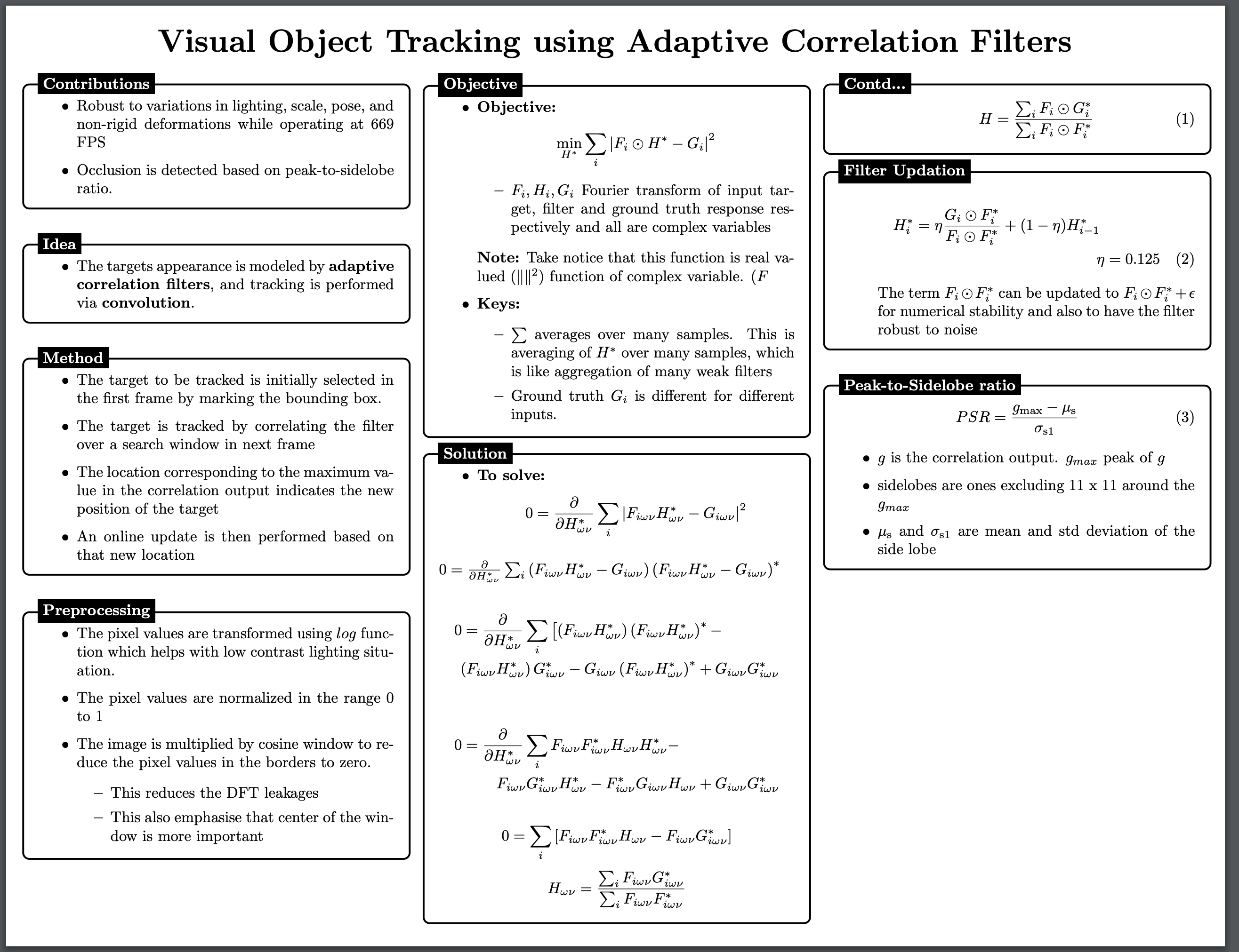
The main idea of the paper is to model the appearance of the target object, frame to frame by constantly updating the correlation filter trained on example images and using the trained filter to update the location of the target in current frame. Correlation filter is trained in Fourier domain which makes it computationally efficient.
Few important aspects of this algorithm is that, it performs well under changes in rotation, scale, lighting and partial occlusion of the target object despite its simplicity.
We go through the code available in the
link
and understand the implementation. Glancing through the code, I found
that good place to start is by understanding MOSSE class
class MOSSE:
    def __init__(self, frame, rect):
        x1, y1, x2, y2 = rect
        w, h = map(cv2.getOptimalDFTSize, [x2-x1, y2-y1])
        x1, y1 = (x1+x2-w)//2, (y1+y2-h)//2
        self.pos = x, y = x1+0.5*(w-1), y1+0.5*(h-1)
        self.size = w, h
        img = cv2.getRectSubPix(frame, (w, h), (x, y))
Constructor __init__of MOSSE class takes frame,rect as inputs, where frame
is the input frame, rect is the initial bounding box input marked by
the user that encloses the object of interest to track in rest of the frames.
The bounding box coordinatesx1, y1, x2, y2 are with respect to the frame.
# map function: map(f, iterable) <==> [f(x) for x in iterable]
w, h = map(cv2.getOptimalDFTSize, [x2-x1, y2-y1])
x1, y1 = (x1+x2-w)//2, (y1+y2-h)//2
cv2.getOptimalDFTSize(vecsize)doc
returns the minimum number N that is greater than equal to vecsize,
so that the DFT of a vector of size N can be processed efficiently.
Here w, h are the updated width and height of the bounding box. Once
we find the new w, h we update the coordinates x1, y1. Rewrite
(x1+x2-w)/2 as (x2-w+x1)/2 to better understand the math this update
self.pos = x, y = x1+0.5*(w-1), y1+0.5*(h-1)
self.size = w, h
img = cv2.getRectSubPix(frame, (w, h), (x, y))
We find the center of bounding box x, y using updated x1, y1, but these co-ordinates are with
respect to the frame. We extract the part of frame which is centered
at x, y with width w and height h using
cv2.getRectSubPixdoc
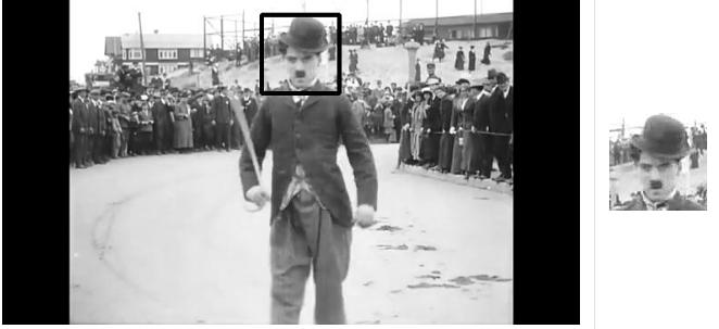
Figure 1.1: Frame with bounding box marked
The next step in the algorithm is to generate the groundtruth for each
input image img, and also preprocess the input.
self.win = cv2.createHanningWindow((w, h), cv2.CV_32F)
g = np.zeros((h, w), np.float32)
g[h//2, w//2] = 1
g = cv2.GaussianBlur(g, (-1, -1), 2.0)
g /= g.max()
self.G = cv2.dft(g, flags=cv2.DFT_COMPLEX_OUTPUT)
self.win = cv2.createHanningWindow((w, h), cv2.CV_32F)
Here cv2.createHanningWindowdoc
generates the hanning windows coefficients of size w, h. The input
image signal is modulated with this function in order to reduce the edge
effects (high frequency).
| Hanning window |
|---|
 |
NOTE::To understand the role of Hanning function, you need to understand the concept of DFT leakage. In short, when we deal with digital signals, if the input signal does not contain frequencies which are integer multiple of analysis frequencies, DFT leakage happens, This can be avoided by modulating the input signal with different window functions such as Hamming, Hanning and rectangular functions before taking Fourier transform
g = np.zeros((h, w), np.float32)
g[h//2, w//2] = 1
g = cv2.GaussianBlur(g, (-1, -1), 2.0)
g /= g.max()
Basic idea of the algorithm is to train correlation filter H*, when
convolved with current input frame should give the new location of the
target. This filter is trained in Fourier domain because its
computationally efficient.
To train, we need input-groundtruth pair. For each img, groundtruth
g is Gaussian shaped peak centered on the target. Above code generates
normalized Gaussian with variance 2.0 as ground truth g for each
input image img
| Ground truth (Gaussian peak) |
|---|
 |
self.G = cv2.dft(g, flags=cv2.DFT_COMPLEX_OUTPUT)
Since we train the filter in Fourier domain, we take the Fourier transform of Gaussian generated in the previous step.
Once we generate the ground truth g, now we generate more training
examples lets call num_images=128 in order to get good initial
estimate of H, which is done by random warping the
input image img using cv2.warpAffinedoc function.
for i in xrange(128):
    a = self.preprocess(rnd_warp(img))
    A = cv2.dft(a, flags=cv2.DFT_COMPLEX_OUTPUT)
    self.H1 += cv2.mulSpectrums(self.G, A, 0, conjB=True)
    self.H2 += cv2.mulSpectrums(     A, A, 0, conjB=True)
self.update_kernel()
self.update(frame)
cv2.warpAffine function needs 2 x 3 transformation matrix T, where top T[:2, :2] is 2 x 2
rotation matrixdoc and T[:, 2] is 2 x 1 is translation matrix.
    a = self.preprocess(rnd_warp(img))

def rnd_warp(a):
    h, w = a.shape[:2]
    T = np.zeros((2, 3))
    coef = 0.2
    ang = (np.random.rand()-0.5)*coef
    c, s = np.cos(ang), np.sin(ang)
    T[:2, :2] = [[c,-s], [s, c]]
    T[:2, :2] += (np.random.rand(2, 2) - 0.5)*coef
    c = (w/2, h/2)
    T[:,2] = c - np.dot(T[:2, :2], c)
    return cv2.warpAffine(a, T, (w, h), borderMode = cv2.BORDER_REFLECT)
The output of warping is shown below
| input image | warped image |
|---|---|
 |
 |
Next step is to preprocess the warped image.
def preprocess(self, img):
    img = np.log(np.float32(img)+1.0)
    img = (img-img.mean()) / (img.std()+eps)
    return img*self.win
During preprocessing, input is transformed using a log function which helps in low contrast
lighting situation, then we normalize the input by subtracting the mean
and dividing by the standard deviation. The input is also modulated
using the hanning window as we discussed before to reduce the edge
effect. The output of the above code is shown below
| input image | log transformed with reduced edge effect# |
|---|---|
|
 |
# image values are normalized between 0-255 for display purpose
Next step includes implementing the equation
 , where
 G is Fourier transform of ground
truth g.
self.H1 += cv2.mulSpectrums(self.G, A, 0, conjB=True)
self.H2 += cv2.mulSpectrums(     A, A, 0, conjB=True)
F is the Fourier transform of input a (in the code F=A)
* indicates the complex conjugate and i indicates the number of
image, which ranges from 1 - 128 in our case
self.H1, self.H2 implements the numerator and denominator part respectively, using the
cv2.mulSpectrumsdoc.
conjB=True option conjugates the second input before mulitplication.
self.update_kernel()

def update_kernel(self):
    self.H = divSpec(self.H1, self.H2)
    self.H[...,1] *= -1

def divSpec(A, B):
    Ar, Ai = A[...,0], A[...,1]
    Br, Bi = B[...,0], B[...,1]
    C = (Ar+1j*Ai)/(Br+1j*Bi)
    C = np.dstack([np.real(C), np.imag(C)]).copy()
    return C
As next step, we get the initial estimation of H*, by calling
self.update_kernel. This function calls divSpec which performs
element wise division grouping real and imaginary part of the data
self.update(frame)

def update(self, frame, rate = 0.125):
    (x, y), (w, h) = self.pos, self.size
    self.last_img = img = cv2.getRectSubPix(frame, (w, h), (x, y))
    img = self.preprocess(img)
    self.last_resp, (dx, dy), self.psr = self.correlate(img)
    self.good = self.psr > 8.0
    if not self.good:
        return

    self.pos = x+dx, y+dy
    self.last_img = img = cv2.getRectSubPix(frame, (w, h), self.pos)
    img = self.preprocess(img)

    A = cv2.dft(img, flags=cv2.DFT_COMPLEX_OUTPUT)
    H1 = cv2.mulSpectrums(self.G, A, 0, conjB=True)
    H2 = cv2.mulSpectrums(     A, A, 0, conjB=True)
    self.H1 = self.H1 * (1.0-rate) + H1 * rate
    self.H2 = self.H2 * (1.0-rate) + H2 * rate
    self.update_kernel()

def correlate(self, img):
    C = cv2.mulSpectrums(cv2.dft(img, flags=cv2.DFT_COMPLEX_OUTPUT), self.H, 0, conjB=True)
    resp = cv2.idft(C, flags=cv2.DFT_SCALE | cv2.DFT_REAL_OUTPUT)
    h, w = resp.shape
    _, mval, _, (mx, my) = cv2.minMaxLoc(resp)
    side_resp = resp.copy()
    cv2.rectangle(side_resp, (mx-5, my-5), (mx+5, my+5), 0, -1)
    smean, sstd = side_resp.mean(), side_resp.std()
    psr = (mval-smean) / (sstd+eps)
    return resp, (mx-w//2, my-h//2), psr
So far, we got the initial estimate of H*. With this H*, we update
the location of target in current frame. This is done by calling the
function correlate.
C = cv2.mulSpectrums(cv2.dft(img, flags=cv2.DFT_COMPLEX_OUTPUT), self.H, 0, conjB=True) correlates the input image with filter.
This is done in Fourier domain again. resp = cv2.idft(C, flags=cv2.DFT_SCALE | cv2.DFT_REAL_OUTPUT) takes
the idft of the FFT output to get the response in spatial domain.
Then, we find the maximum response and its location using cv2.minMaxLocdoc in the line _, mval, _, (mx, my) = cv2.minMaxLoc(resp)
We then calculate Peak-Sidelobe-Ratio (PSR), which is given by PSR =
(mval - mean_side_lobe) / std_side_lobe, where mval is maximum response.
The side lobe considered is 11x11 pixel around (mx, my)
psr = (mval-smean) / (sstd+eps). eps=1e-5 is used for numerical stability.
If psr <= 8.0, then the object is considered to be occluded or
tracking has failed.
self.H1 = self.H1 * (1.0-rate) + H1 * rate
self.H2 = self.H2 * (1.0-rate) + H2 * rate
self.update_kernel()
Once we got the location self.pos of target for the current frame, we
update our estimate H* by calculating self.H1 and self.H2 and
updating the filter with learning rate of 0.125. This continues for
each frame where we update the filter and the location of target hand in
hand.
Thats how tracking using correlation filter is done!. Hope you could understand the algorithm better. Thank you for reading.
Summary of the paper:
Summary of the method